Simulation Example for Spinach • AquacropOnR

This is a basic example to run AquaCrop from R for the spinach crop.

Importantly, the working directory should be set to the folder in which the aquacrop.exe file is located. This path should also contain no spaces. For example: path_to_aquacrop_folder <- "C:/users/username/AquaCrop71/".

library(AquacropOnR)
library(tidyverse)
setwd(dir = path_to_aquacrop_folder)

With the package comes an example list with default crop parameters for quinoa and spinach. To make this list for your own crop, you need an AquaCrop cropfile (YourCrop.CRO) whose path should be input in the read_CRO() function:

yourcrop <- read_CRO("path/YourCrop.CRO")`

Once you have the list with default crop parameter values, you can design the scenario’s for which you want to run AquaCrop. The AquacropOnR package provides a function to design the scenario’s: design_scenario(). The arguments in this function have the following meaning:

name is a character vector of names for the scenario’s.
Input_Date is a Date vector that indicates the start point of the meteo files (Plu, Tnx, ETo).
Sim_Date is a Date vector that indicates the start point of the simulation in each scenario.
Plant_Date is a Date vector that defines the planting date in each scenario.
IRRI is a character vector of the names of the irrigation scenario’s present in the ID column of the IRRI_s tibble.
Soil is a character vector of the names of the soils present in the ID column of the SOL_s tibble.
Plu, Tnx, and ETo are character (vectors) that refer to the names of R objects, that hold the daily data for precipitation, temperature and reference evapotranspiration, respectively.
FMAN is a character vector of the names of the management scenario’s present in the ID column of the FMAN_s tibble.
SW0 is a character vector of the names of the initial condition scenario’s present in the ID column of the SW0_s tibble.
GWT is a numeric vector of values for the depth of the Ground Water Table (in m), for each scenario.

IMPORTANT:

The Scenario_s tibble must be named Scenario_s and must have the columns (variables) Scenario, Input_Date, Plant_Date, IRRI, Soil and Meteo. Other arguments Sim_Date, FMAN, GWT and SW0 have default values if not provided explicitly. See design_scenario().
The irrigation tibble must be named IRRI_s and must have the columns ID, Timing, Depth and ECw. Values of the ID column are given as input to the IRRI argument in the design_scenario() function.
The soil tibble must be named SOL_s and must have the columns ID, Horizon, Thickness, SAT, FC, WP, Ksat, Penetrability and Gravel. Values of the ID column are given as input to the Soil argument in the design_scenario() function.
The precipitation tibble can be named as you want, but its name is the input to the Plu argument in the design_scenario() function. This tibble must have the columns DAY and PLU.
The reference evapotranspiration tibble can be named as you want, but its name is the input to the ETo argument in the design_scenario() function. This tibble must have the columns DAY and ETo.
The temperature tibble can be named as you want, but its name is the input to the Tnx argument in the design_scenario() function. This tibble must have the columns DAY, TMAX and TMIN.
The Management tibble must be named FMAN_s and must have the columns ID, mulch_perc, mulch_eff, fert_stress, soil_bunds, runoff_aff, CN_eff, weed_clo, weed_mid, weed_cc.
The initial conditions tibble must be named SW0_s, and must contain the columns ID, Horizon, Thickness, WC and ECe.

Examples of these tibbles are available from the package.

The default FMAN_s tibble associated to the package looks like this:

#> # A tibble: 1 × 10
#>   ID      mulch_perc mulch_eff fert_stress soil_bunds runoff_aff CN_eff weed_clo
#>   <chr>        <dbl>     <dbl>       <dbl>      <dbl>      <dbl>  <dbl>    <dbl>
#> 1 default          0        50           0          0          0      0        0
#> # ℹ 2 more variables: weed_mid <dbl>, weed_cc <dbl>

but you can create your own, as long as it has the same column names, and is named FMAN_s.
The default IRRI_s tibble associated to the package looks like this:

#> # A tibble: 2 × 4
#>   ID       Timing Depth   ECw
#>   <chr>     <dbl> <dbl> <dbl>
#> 1 no_irrig     20     0     0
#> 2 simple       20    25     0

We can make a new irrigation input tibble as follows:

IRRI_s <- IRRI_s %>% 
  bind_rows(tibble(ID = c("IRRI_01", "IRRI_01"), Timing = c(20, 35), Depth = c(25,25), ECw = c( 0, 0)))

which looks like:

#> # A tibble: 4 × 4
#>   ID       Timing Depth   ECw
#>   <chr>     <dbl> <dbl> <dbl>
#> 1 no_irrig     20     0     0
#> 2 simple       20    25     0
#> 3 IRRI_01      20    25     0
#> 4 IRRI_01      35    25     0

For this example we will use the data for soil, precipitation, temperature and reference evapotranspiration that comes with the package. These tibbles should be formatted as presented below.

#> # A tibble: 1 × 9
#>   ID      Horizon Thickness   SAT    FC    WP  Ksat Penetrability Gravel
#>   <chr>     <dbl>     <dbl> <dbl> <dbl> <dbl> <dbl>         <dbl>  <dbl>
#> 1 Soil_01       1         4    41    22    10  1200           100      0
#> # A tibble: 6 × 2
#>     DAY   PLU
#>   <dbl> <dbl>
#> 1     1   0.4
#> 2     2   0.7
#> 3     3   0.8
#> 4     4   0.2
#> 5     5   0  
#> 6     6   0.3
#> # A tibble: 6 × 3
#>     DAY  TMAX  TMIN
#>   <dbl> <dbl> <dbl>
#> 1     1   9.3   7.2
#> 2     2   7.4   5  
#> 3     3   6.8   2.1
#> 4     4   6.5   2.5
#> 5     5   6.5   2.9
#> 6     6   7.4   4.3
#> # A tibble: 6 × 2
#>     DAY   ETo
#>   <dbl> <dbl>
#> 1     1 1.03 
#> 2     2 1.17 
#> 3     3 0.743
#> 4     4 0.887
#> 5     5 0.778
#> 6     6 0.695

Scenario_s <- design_scenario(name = c("S_01", "S_02"),
                              Input_Date = as.Date("2019-01-01"),
                              Plant_Date = as.Date(c("2019-04-01", "2019-04-01")), 
                              IRRI = c("no_irrig", "IRRI_01"),
                              Soil = "Soil_01", 
                              Plu = "Plu_01",
                              Tnx = "Tnx_01",
                              ETo = "ETo_01",
                              FMAN = "default",
                              GWT = 2.0)

The Scenario_s tibble should look like this:

#> # A tibble: 2 × 12
#>   Scenario Input_Date Sim_Date   Plant_Date IRRI   Soil  Plu   Tnx   ETo   FMAN 
#>   <chr>    <date>     <date>     <date>     <chr>  <chr> <chr> <chr> <chr> <chr>
#> 1 S_01     2019-01-01 2019-04-01 2019-04-01 no_ir… Soil… Plu_… Tnx_… ETo_… defa…
#> 2 S_02     2019-01-01 2019-04-01 2019-04-01 IRRI_… Soil… Plu_… Tnx_… ETo_… defa…
#> # ℹ 2 more variables: GWT <dbl>, SW0 <chr>

Then it is crucial to create the correct AquaCrop path, while checking the required folders and choosing which daily outputs to produce. Therefore the package has the function path_config(). Make sure your path ends with a “/”. For example: path_to_aquacrop_folder <- "C:/users/username/AquaCrop71/".

AQ <- path_config(AquaCrop.path = path_to_aquacrop_folder)

Finally, we can run AquaCrop using the aquacrop_wrapper() function and display a plot. The param_values argument is used to modify crop parameters from the default, which is the list provided as input to the defaultpar argument inside the model_options list. situation takes a vector of characters, that correspond to the Scenario variable in the Scenario_s tibble. The daily_output argument lets you choose which output type to return from the simulation (see Codes in AquaCrop manual p21-25). The output argument in the model_options defines the output format of the simulation. If "croptimizr", the result is a list, ready to use in the CroptimizR package. If anything else, the result is a tibble.

Let us first run the simulation with the default parameters for spinach:


default <- aquacrop_wrapper(param_values = list(),
               situation = c("S_01","S_02"),               
               model_options = list(AQ = AQ, cycle_length = 70,
                                    defaultpar = Spinach, output = "df", 
                                    daily_output = c(1,2)))

ggplot(mapping = aes(x=DAP, y=Biomass)) +
  # ylim(0, 3.5) +
  geom_line(data = default, aes(group = Scenario, color = Scenario),linewidth = 1) +
  geom_text(aes(x=40, y=3, label = 'default'), color = "black") +
  xlim(0, 70) +
  scale_color_manual(values = c("black", "red")) +
  theme_bw()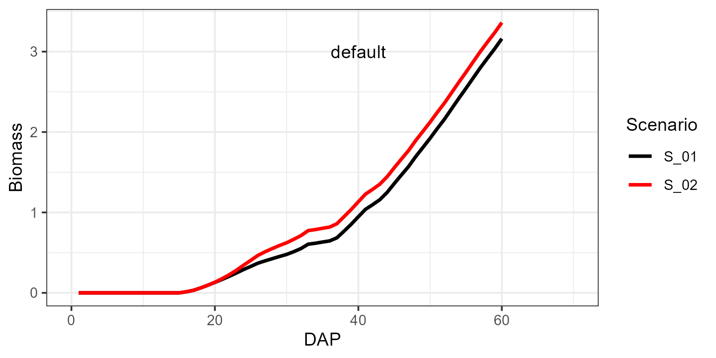

And now let’s see what happens when we increase the canopy growth coefficient cgc from 0.15 to 0.18:

modified <- aquacrop_wrapper(param_values = list(cgc = 0.18),
               situation = c("S_01", "S_02"),
               model_options = list(AQ = AQ, cycle_length = 70,
                                    defaultpar = Spinach, output = "df", 
                                    daily_output = c(1,2)))

ggplot() +
  ylim(0, 3.5) +
  geom_line(data = default, aes(x=DAP, y=Biomass, group = Scenario, color = Scenario),linewidth = 1) +
  geom_line(data = modified, aes(x=DAP, y=Biomass, group = Scenario, color = Scenario),linewidth = 1, linetype = 2) +
  geom_text(aes(x=40, y=3, label = 'default'), color = "black", hjust = 0) +
  geom_text(aes(x=40, y=2.8, label = 'modified'), color = "black", hjust = 0) +
  geom_segment(mapping = aes(x = 34, xend = 39, y = 3, yend = 3), color = 'black', linewidth = 1, linetype = 1) +
  geom_segment(mapping = aes(x = 34, xend = 39, y = 2.8, yend = 2.8), color = 'black', linewidth = 1, linetype = 2) +
  xlim(0, 70) +
  scale_color_manual(values = c("black", "red")) +
  theme_bw()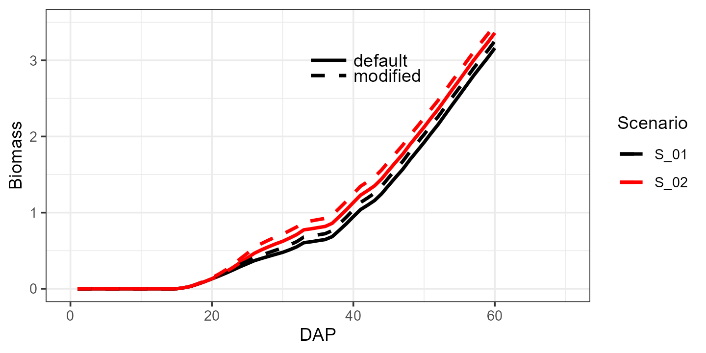

A list of parameters with their explanation can be found in the vignette("crop-parameters").